Lithology Prediction Using Deep Learning: Force 2020 Dataset: Part.1 (data visualization)
- Ryan Mardani
- Mar 2, 2021
- 3 min read
The objective of the Force 2020 competition was to predict lithology labels from well logs, provided NDP lithostratigraphy and well X, Y position. In this work, it is attempted to have a standard approach, like other Machine Learning problems, to improve prediction scores using Deep Learning methodology. The dimension of the dataset is pretty large and for training purposes, we should consider calculation costs limitations. To tackle this problem, we can get benefit from the parallel calculation in GPU using the TensorFlow library. As we will build an almost large neural network (several hidden dense layers ), GPU calculation can speed up the training process at least ten times than CPU training mode. Before doing anything, we need to get familiar with the dataset. You can access the full data download link from here.
See the GitHub account for source codes used in this post.
Dataset:
It contains 118 well data in total, 98 aimed for training, 10 for testing, and the rest as blind well data from offshore Norway. In addition, well coordinates and interpreted lithofacies and lithostratigraphy, these well log measurements are also included: CALI, RDEP, RHOB, DHRO, SGR, GR, RMED, RMIC, NPHI, PEF, RSHA, DTC, SP, BS, ROP, DTS, DCAL, MUDWEIGHT. Except for GR and depth, other logs have missing values and will be taken care of in the data preparation process. For detailed data explanation, you may read more from here.
In the part.1, well locations map, well logs, and some important cross plots will be plotted like conventional petrophysical methods to let the user get familiar with the dataset. Before that, we should download LAS files and read them into the disk in Python. If you are a novice at working with LAS files in the Python environment, I invite you to read my first and second posts that can be helpful for this topic.
Although for the competition the training and test datasets were provided in .csv format as a single file, here, we would prefer to deal with LAS files and the formation tops. For comparability, we will consider the same wells as train and test wells in competition.
Well Data Distribution:
In the figure below, geographical well locations are plotted using X and Y coordinates in the circle shape. Circle sizes are proportional to available data points for that specific well. This does not mean wells with bigger circles contains more various well logs, possibly logged longer intervals.
It is clear that we are dealing with almost three clusters of wells, NW, SW, and NE. We can see that test wells are chosen fairly consistent with whole data points distribution. We will cover more in the next parts. Train wells are in red, test in blue, and blind wells in green.

Well Log Plot:
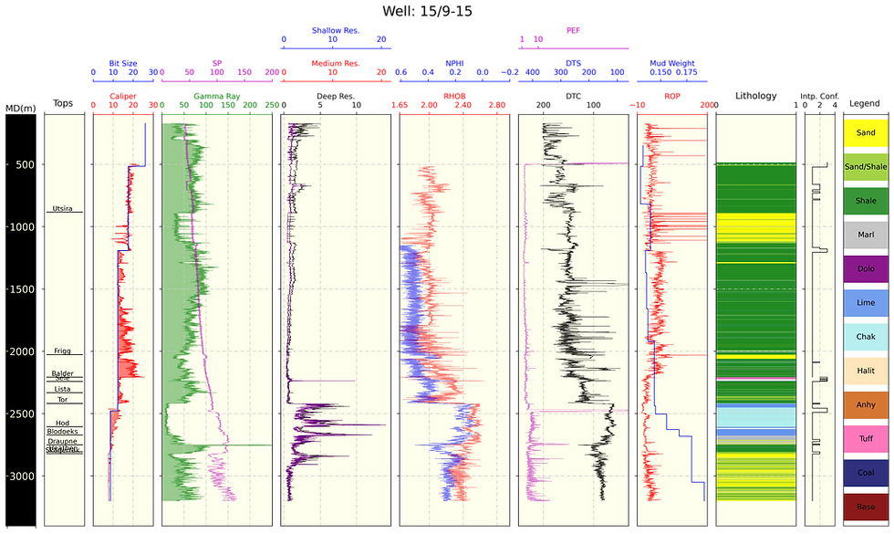
The most important and frequent well logs are plotted (in the figure below) for an individual well. You may call log_plots(well_name, start_depth , stop_depth) to visualize your favorite wells. In fact, this kind of plot is one of the most qualitative approaches for your well data. You may examine noise level, the correlation between various logs, availability, or absence of a specific log. To understand the dataset, it is recommended to browse each well carefully. Beyond, quantitative approaches for feature selection, sometimes, visual judgment can be helpful.

Cross Plots:
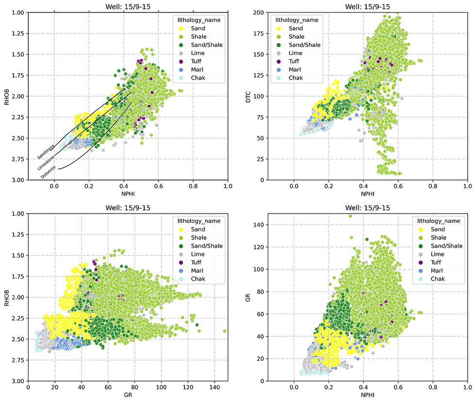
Cross plots can be an important visualization tool for data correlation and variable relationships. For this dataset with 16 features (logs), we can plot more than 3500 unique cross plots while it is not a reasonable approach. We should consider those logs that petrophysically have meaningful relationships. Gamma Ray, Sonic, Density, and Neutron porosity show a great correlation with the meaningful grouping of lithology types.

In the next part of this work, we will cover exploratory data analysis, data manipulation, and preparation for modeling.
Please contact for any questions or more details: ryan.mardani@dataenergy.ca

Comments